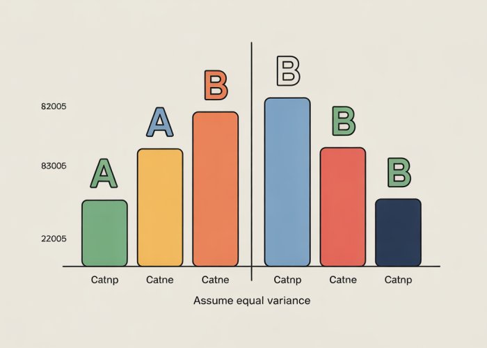
The Student’s t-test, a staple in statistical hypothesis testing, often hinges on critical assumptions. One such assumption is homoscedasticity, which dictates that different populations have the same variance. When conducting a t-test, researchers must decide whether to assume equal variance; this decision heavily influences the calculation and interpretation of results. SPSS, a widely used statistical software package, provides options for both assuming equal variances and adjusting for unequal variances, necessitating a clear understanding of the implications. Choosing the correct t-test variant requires careful consideration of the data and a thorough understanding of assume equal variance.
The T-Test stands as a cornerstone of statistical analysis, a workhorse employed across disciplines to discern whether a significant difference exists between the means of two groups. From clinical trials evaluating drug efficacy to marketing campaigns assessing customer engagement, the T-Test provides a framework for drawing meaningful conclusions from data.
Its widespread adoption underscores its utility, but also necessitates a thorough understanding of its underlying assumptions. Chief among these is the assumption of equal variances, a principle often overlooked yet crucial for the validity of the test.
This editorial delves into the intricacies of this assumption, aiming to illuminate its importance and the potential pitfalls of its violation.
The Ubiquitous T-Test: A Brief Overview
At its core, the T-Test is a hypothesis test designed to determine if there’s a statistically significant difference between the averages of two independent groups. We are trying to understand if the difference we observe in our sample data is a real difference in the overall population or just due to random chance.
It achieves this by calculating a t-statistic, which reflects the magnitude of the difference between the group means relative to the variability within the groups. This statistic is then compared to a t-distribution to obtain a p-value, which indicates the probability of observing such a difference if there were truly no difference between the populations.
A small p-value (typically less than 0.05) suggests strong evidence against the null hypothesis (the hypothesis of no difference), leading to the conclusion that the means are indeed different.
Equal Variance: The Unsung Hero
The T-Test, in its most common form (Student’s t-test), operates under the assumption that the two groups being compared have approximately equal variances. Variance, in this context, refers to the spread or dispersion of data points around the mean.
Essentially, it assumes that the variability within each group is similar. Why is this important? Because the T-Test uses a pooled variance estimate to calculate the t-statistic.
This pooled estimate is only accurate if the variances are truly equal.
The Goal: Unpacking the Equal Variance Assumption
This editorial sets out to demystify the equal variance assumption, providing a comprehensive exploration of its implications for T-Test analysis. Our primary objective is to explain why this assumption matters and how it can influence the results of your statistical tests.
By clarifying the concept of equal variance, differentiating it from unequal variance (heteroscedasticity), and outlining methods for assessing its validity, we aim to empower you to conduct more robust and reliable T-Tests.
Consequences of Assumption Violation: A Sneak Peek
Ignoring the equal variance assumption can have serious consequences. If the variances are unequal and this is not accounted for, the p-values generated by the T-Test may be inaccurate.
This can lead to an increased risk of Type I errors (false positives), where you incorrectly conclude that a significant difference exists when, in reality, it does not. Understanding these potential pitfalls is essential for making informed decisions based on T-Test results.
The Ubiquitous T-Test: A Brief Overview
At its core, the T-Test is a hypothesis test designed to determine if there’s a statistically significant difference between the averages of two independent groups. We are trying to understand if the difference we observe in our sample data is a real difference in the overall population or just due to random chance.
It achieves this by calculating a t-statistic, which reflects the magnitude of the difference between the group means relative to the variability within the groups. This statistic is then compared to a t-distribution to obtain a p-value, which indicates the probability of observing such a difference if there were truly no difference between the populations.
A small p-value (typically less than 0.05) suggests strong evidence against the null hypothesis (the hypothesis of no difference), leading to the conclusion that the means are indeed different. However, before jumping to conclusions based solely on the p-value, it’s important to consider the underlying assumptions of the T-Test, which will be explored in later sections.
T-Test Fundamentals: A Quick Overview
Before diving deeper into the intricacies of equal variance, it’s crucial to solidify our understanding of the T-Test itself. This statistical tool, while powerful, operates under specific principles and comes in various forms. A clear grasp of these fundamentals is essential for correctly applying and interpreting the T-Test.
Unveiling the Underlying Principles
The T-Test, in essence, is a method for comparing the means of two groups. But what does this comparison truly entail?
It involves calculating a t-statistic, which quantifies the difference between the means relative to the variability within each group. Think of it as a signal-to-noise ratio: a larger t-statistic suggests a stronger signal (difference between means) compared to the noise (variability within groups).
This t-statistic is then evaluated against a t-distribution, a probability distribution that allows us to determine the likelihood of observing such a t-statistic if there were truly no difference between the population means. This likelihood is quantified by the p-value.
Navigating the T-Test Landscape: Different Types
The T-Test isn’t a one-size-fits-all solution. It comes in several flavors, each designed for specific scenarios. Two of the most common types are the independent samples T-Test and the paired samples T-Test.
Independent Samples T-Test
The independent samples T-Test (also known as the two-sample T-Test) is used to compare the means of two unrelated groups. For example, you might use this test to compare the effectiveness of a new drug to a placebo group, where the individuals in each group are distinct and unrelated.
Paired Samples T-Test
In contrast, the paired samples T-Test (also known as the dependent samples T-Test) is used when comparing the means of two related groups. This often involves measuring the same subject twice under different conditions. A classic example is measuring a patient’s blood pressure before and after taking a medication.
The key distinction is whether the data points in the two groups are related or independent. Choosing the correct type of T-Test is paramount for obtaining accurate results.
Demystifying Hypothesis Testing: Key Concepts
The T-Test is rooted in the framework of hypothesis testing, a systematic approach to making inferences about populations based on sample data. Several key concepts are essential for understanding this process.
Null Hypothesis
The null hypothesis represents the default assumption: that there is no difference between the population means. The T-Test aims to assess whether there is sufficient evidence to reject this null hypothesis.
Alternative Hypothesis
The alternative hypothesis is the statement we’re trying to find evidence for. It contradicts the null hypothesis and suggests that there is a difference between the population means.
P-value
The p-value is the probability of observing the obtained results (or more extreme results) if the null hypothesis were true. A small p-value suggests that the observed data is unlikely to have occurred by chance alone if there’s no real difference.
Statistical Significance
Statistical significance is a threshold used to determine whether the p-value is small enough to reject the null hypothesis. This threshold is typically set at 0.05, meaning that if the p-value is less than 0.05, we reject the null hypothesis and conclude that there is a statistically significant difference between the means.
Understanding these fundamental concepts is crucial for correctly interpreting the results of a T-Test and drawing meaningful conclusions from your data.
The T-Test, in essence, is a method for comparing the means of two groups. But what does this comparison truly entail?
It involves assessing whether the observed difference between sample means is large enough to suggest a real difference in the population means, rather than just random variation. The validity of this assessment, however, hinges on certain assumptions, one of the most crucial being the assumption of equal variance.
Unveiling the Equal Variance Assumption (Homoscedasticity)
At the heart of many statistical analyses lies a set of assumptions. These assumptions, often unseen and unspoken, are the silent pillars upon which the validity of our conclusions rests.
One such pillar, particularly relevant to the T-Test, is the assumption of equal variance, also known as homoscedasticity.
Defining Equal Variance: A State of Uniformity
In simple terms, equal variance means that the spread or dispersion of data points around the mean is roughly the same for both groups being compared.
Imagine two classrooms taking the same test. Equal variance would imply that the scores in both classrooms are scattered similarly around their respective averages. Neither classroom exhibits a much wider or narrower range of scores than the other.
Mathematically, this translates to the variances of the two populations being equal. Variance, you might recall, is a measure of how much the data points deviate from the mean.
Homoscedasticity vs. Heteroscedasticity: A Tale of Two Distributions
The opposite of homoscedasticity is heteroscedasticity, or unequal variance. In this scenario, the spread of data differs significantly between the groups.
Returning to our classroom analogy, heteroscedasticity would occur if one classroom’s scores were tightly clustered around the average, while the other classroom’s scores were widely dispersed, spanning a much larger range.
Visually, if you were to plot the data, heteroscedasticity might manifest as a funnel shape, where the spread of the data increases (or decreases) as you move along the x-axis.
Why Equal Variance Matters: The Foundation of a Valid T-Test
The assumption of equal variance is not merely a technical detail; it’s a critical foundation for the standard T-Test.
The T-Test relies on a pooled variance estimate, which combines the variances of the two groups into a single estimate of the population variance. This pooled estimate is used to calculate the t-statistic, which in turn determines the p-value.
When variances are unequal, this pooled estimate becomes unreliable. It can either underestimate or overestimate the true variance, leading to inaccurate t-statistics and p-values.
Specifically, if the group with the larger variance also has a larger sample size, the standard T-Test can be overly liberal, increasing the risk of a Type I error (falsely rejecting the null hypothesis).
Conversely, if the group with the smaller variance has a larger sample size, the T-Test can be overly conservative, increasing the risk of a Type II error (failing to reject a false null hypothesis).
In essence, violating the equal variance assumption can distort the T-Test’s ability to accurately assess the difference between group means, leading to potentially misleading conclusions. Therefore, before relying on the results of a T-Test, it’s imperative to assess whether this assumption holds true.
The tale of two distributions – one exhibiting uniformity, the other disparity – underscores why we can’t blindly apply the T-Test. But how do we objectively determine if our data meets the crucial assumption of equal variance? Fortunately, statistical tools exist to help us "test the waters" before diving into our analysis.
Testing the Waters: Assessing Equal Variance with Levene’s Test
Levene’s Test stands as a sentinel, guarding against the perils of violating the equal variance assumption. It is a statistical procedure designed to specifically assess whether two or more groups have equal variances. Understanding how Levene’s Test works and how to interpret its results is crucial for ensuring the validity of your T-Test.
Introducing Levene’s Test: The Variance Detective
Levene’s Test, in essence, examines whether the variance of a variable is equal across different groups. Unlike some other tests that are highly sensitive to departures from normality, Levene’s Test is more robust, meaning it performs reasonably well even when the data is not perfectly normally distributed.
This robustness makes it a preferred choice for assessing equal variance in many situations, particularly when dealing with real-world data that often deviates from theoretical ideals.
How Levene’s Test Works: Unmasking Variance Differences
The mechanics of Levene’s Test involve a clever transformation of the original data. Instead of directly comparing the variances of the groups, Levene’s Test focuses on the absolute deviations from the group means (or medians, in some variations of the test).
Here’s a simplified breakdown:
-
Calculate the absolute deviation of each data point from its group mean (or median).
-
Perform an Analysis of Variance (ANOVA) on these absolute deviations.
-
Examine the resulting p-value from the ANOVA.
The null hypothesis of Levene’s Test is that the population variances are equal. A small p-value (typically less than 0.05) indicates that there is significant evidence to reject the null hypothesis. In other words, a significant p-value suggests that the variances are unequal.
Conversely, a non-significant p-value (greater than 0.05) suggests that we do not have sufficient evidence to reject the null hypothesis of equal variances.
It’s important to remember that failing to reject the null hypothesis does not prove that the variances are equal; it simply means that we don’t have enough evidence to conclude that they are different.
Interpreting Levene’s Test Results: A Decision Point
The p-value obtained from Levene’s Test is the key to making an informed decision about whether to proceed with a standard T-Test or to consider alternative approaches.
-
Significant p-value (p < 0.05): Unequal variances are likely present. You should not use the standard T-Test. Instead, consider Welch’s T-Test (discussed later) or other methods suitable for unequal variances.
-
Non-significant p-value (p > 0.05): Equal variances can be assumed. You can proceed with the standard T-Test, keeping in mind that the test is based on this assumption.
Careful interpretation of Levene’s Test is essential to avoid drawing incorrect conclusions from your T-Test analysis.
The F-Test: An Alternative Glimpse
While Levene’s Test is widely used, the F-test offers another avenue for comparing variances between two groups. The F-test directly compares the ratio of the two variances.
However, the F-test is highly sensitive to departures from normality, making it less robust than Levene’s Test in many real-world scenarios. Therefore, Levene’s Test is generally preferred, especially when the data’s normality is questionable.
The Levene’s Test might reveal that our assumption of equal variances is, unfortunately, not met. This isn’t necessarily a roadblock to our analysis, but rather a signpost directing us toward a more appropriate statistical tool. When faced with unequal variances, we can’t simply ignore the problem. Doing so can lead to flawed conclusions.
Remedial Action: Addressing Unequal Variance with Welch’s T-Test
So, what happens when Levene’s Test throws a wrench in the works, indicating unequal variances between our groups? Do we abandon the T-Test altogether? Fortunately, no. We have a powerful alternative at our disposal: Welch’s t-test.
Welch’s t-test is specifically designed to handle situations where the assumption of equal variances is violated. It’s a modification of the standard T-Test that provides a more accurate comparison of means when the variances are unequal.
Why Welch’s T-Test is a Superior Choice
The key advantage of Welch’s t-test lies in its robustness. Unlike the standard T-Test, it doesn’t assume equal variances. This makes it a more reliable choice when dealing with data that exhibits heteroscedasticity (unequal variances).
By using Welch’s t-test, we can avoid the inflated Type I error rates and inaccurate p-values that can result from applying a standard T-Test to data with unequal variances.
The Magic of Adjusted Degrees of Freedom
The core of Welch’s t-test’s effectiveness lies in its adjustment of the degrees of freedom.
Degrees of freedom, in essence, represent the amount of independent information available to estimate a parameter. In the context of the T-Test, they influence the shape of the t-distribution, which in turn affects the p-value.
When variances are unequal, the standard calculation of degrees of freedom becomes inaccurate. Welch’s t-test employs a more complex formula to estimate the degrees of freedom, taking into account the differing variances and sample sizes of the groups being compared. This adjusted degrees of freedom value leads to a more accurate p-value, reflecting the true difference between the means of the groups.
Beyond Welch’s: Other Avenues to Explore
While Welch’s t-test is often the go-to solution for unequal variances, it’s worth noting that other options exist.
Data transformations can sometimes stabilize variances, making the standard T-Test applicable. Common transformations include logarithmic, square root, or reciprocal transformations. However, transformations can alter the interpretation of the data, so they should be used cautiously.
Non-parametric tests, such as the Mann-Whitney U test, offer another alternative. These tests don’t rely on assumptions about the distribution of the data or the equality of variances. However, they may be less powerful than parametric tests like the T-Test when the assumptions of the T-Test are met.
Ultimately, the choice of which method to use depends on the specific characteristics of your data and the research question you’re trying to answer. However, when Levene’s Test signals unequal variances, Welch’s t-test should be a primary consideration.
Interpreting the Results: A Comprehensive Guide
Welch’s t-test offers a robust solution when the assumption of equal variances is violated. But simply running the test is not enough. Understanding how to interpret the results, and how those results differ based on whether you’ve used a standard T-Test or Welch’s modification, is crucial for drawing accurate conclusions from your data.
Variance Checks First, Interpretations Second
The golden rule of T-Tests is: always assess the equal variance assumption before diving into the T-Test results. This is not merely a procedural step; it fundamentally affects how you interpret the output.
If Levene’s Test (or a similar test) indicates equal variances, you can confidently interpret the results of the standard Independent Samples T-Test. If, however, the assumption is violated, you must rely on the Welch’s T-Test output.
Mixing these up can lead to serious misinterpretations and flawed conclusions.
Reporting Results: Two Paths Diverge
The way you report your T-Test findings will differ depending on whether you assumed equal variances or used Welch’s T-Test.
Reporting with Assumed Equal Variances
When equal variances are assumed, you’ll report the following:
- The t-statistic.
- Degrees of freedom (df) from the standard T-Test output.
- The p-value.
- The means and standard deviations for each group.
- A confidence interval for the difference in means.
Example: "An independent samples t-test revealed a significant difference in mean scores between Group A (M = X, SD = Y) and Group B (M = Z, SD = W), t(df) = value, p = value, 95% CI [lower bound, upper bound]."
Reporting with Welch’s T-Test
When using Welch’s T-Test due to unequal variances, you’ll report similar statistics, but with a critical distinction:
- The t-statistic from Welch’s T-Test.
- Welch’s degrees of freedom (which will likely be a non-integer value).
- The p-value from Welch’s T-Test.
- The means and standard deviations for each group.
- A confidence interval for the difference in means.
Example: "Welch’s t-test indicated a significant difference in mean scores between Group A (M = X, SD = Y) and Group B (M = Z, SD = W), t(Welch’s df) = value, p = value, 95% CI [lower bound, upper bound]."
Note the explicit mention of "Welch’s" before the degrees of freedom. This is crucial for clarity and transparency.
Connecting Findings to the Null Hypothesis
Ultimately, the goal of a T-Test is to determine whether there is enough evidence to reject the null hypothesis.
-
The null hypothesis typically states that there is no difference in means between the two groups.
-
The alternative hypothesis states that there is a difference.
The p-value provides the key to this decision.
-
If the p-value is less than your chosen significance level (alpha, typically 0.05), you reject the null hypothesis and conclude that there is a statistically significant difference between the group means.
-
If the p-value is greater than alpha, you fail to reject the null hypothesis, indicating that there is not enough evidence to conclude a significant difference.
Remember: Failing to reject the null hypothesis does not mean that there is no difference. It simply means that you haven’t found sufficient evidence to demonstrate one.
Always state your conclusion in the context of your research question. For example: "Based on Welch’s t-test, we found a statistically significant difference in [variable of interest] between [Group A] and [Group B], suggesting that [interpretation related to your research question]."
Real-World Applications: Case Studies and Examples
Having explored the theoretical underpinnings and practical implications of the equal variance assumption, it’s time to ground these concepts in real-world scenarios. By examining concrete examples, we can solidify our understanding of how to apply the T-Test correctly and interpret its results in diverse contexts.
This section will delve into several case studies, demonstrating how to perform the T-Test and Levene’s Test, and critically, how to choose between the standard T-Test and Welch’s T-Test based on the variance assessment.
Case Study 1: Comparing Website Conversion Rates
Imagine an e-commerce company testing two different website designs to see which one leads to higher conversion rates. They randomly split their website traffic, directing half to Design A and half to Design B. After a week, they collect data on the conversion rates for each group.
The critical question: Is there a statistically significant difference in conversion rates between the two designs?
Step 1: Data Collection and Preparation
First, the company needs to collect data on the conversion rates for both website designs. This involves calculating the percentage of visitors who made a purchase under each design.
Data cleaning and preparation are crucial steps to ensure data accuracy and consistency.
Step 2: Assessing Equal Variance with Levene’s Test
Before running the T-Test, we must check the equal variance assumption. Using statistical software, perform Levene’s Test on the conversion rate data for Design A and Design B.
If Levene’s Test yields a p-value greater than 0.05 (or a chosen alpha level), we can assume equal variances.
This means we can proceed with the standard Independent Samples T-Test.
However, if the p-value is less than 0.05, we reject the null hypothesis of equal variances and must use Welch’s T-Test instead.
Step 3: Performing the Appropriate T-Test
Based on the outcome of Levene’s Test, we perform either the standard Independent Samples T-Test or Welch’s T-Test. The software will provide a t-statistic, degrees of freedom, p-value, and confidence interval.
Step 4: Interpreting the Results
Let’s assume Levene’s Test indicated unequal variances, leading us to use Welch’s T-Test. Suppose Welch’s T-Test yields a p-value of 0.03. This indicates a statistically significant difference in conversion rates between Design A and Design B.
Because the p-value (0.03) is less than the conventional alpha level of 0.05, we reject the null hypothesis.
Furthermore, examining the sample means reveals that Design B has a higher conversion rate. Thus, we can conclude that Design B is significantly more effective at driving conversions than Design A.
Case Study 2: Evaluating the Effectiveness of a New Drug
A pharmaceutical company is testing a new drug to lower blood pressure. They conduct a clinical trial, randomly assigning participants to either a treatment group (receiving the new drug) or a control group (receiving a placebo).
After several weeks, they measure the blood pressure of each participant. The goal: Determine if the new drug is significantly more effective than the placebo in lowering blood pressure.
Step 1: Data Collection and Preparation
Collect blood pressure measurements for both the treatment and control groups.
Ensure the data is properly cleaned and formatted for statistical analysis.
Step 2: Checking the Equal Variance Assumption
Apply Levene’s Test to the blood pressure data from both groups. Assume, in this case, that Levene’s Test indicates equal variances (p > 0.05).
Therefore, we can proceed with the standard Independent Samples T-Test.
Step 3: Running the Independent Samples T-Test
Perform the Independent Samples T-Test using statistical software. The output will include the t-statistic, degrees of freedom, p-value, and confidence interval.
Step 4: Interpreting the Results
Suppose the Independent Samples T-Test results in a p-value of 0.10. This means there’s no statistically significant difference in blood pressure between the treatment and control groups.
The p-value (0.10) is greater than the common alpha level of 0.05. Therefore, we fail to reject the null hypothesis.
Even if the treatment group shows a slightly lower average blood pressure, the difference is not statistically significant. We can conclude that the new drug is not demonstrably more effective than the placebo in lowering blood pressure, based on this study.
Choosing the Right T-Test: A Recap
These case studies highlight the importance of assessing the equal variance assumption before performing a T-Test. Levene’s Test acts as a gatekeeper, guiding us towards the appropriate T-Test.
- Equal Variances (Levene’s Test p > 0.05): Use the standard Independent Samples T-Test.
- Unequal Variances (Levene’s Test p < 0.05): Use Welch’s T-Test.
By diligently following this process, we can ensure more accurate and reliable results in our statistical analyses.
T-Test: Assume Equal Variance? Frequently Asked Questions
Confused about when to assume equal variance in a t-test? These frequently asked questions provide quick answers to common concerns.
What does "assume equal variance" actually mean in a t-test?
"Assume equal variance" (also known as homogeneity of variance) means you believe that the populations your two samples are drawn from have approximately the same amount of variability. This is a key assumption for the independent samples t-test. If this assumption holds, you can use the pooled variance t-test.
How do I know if I can assume equal variance for my t-test?
You can use statistical tests like Levene’s test or Bartlett’s test to formally check for equal variances. These tests produce a p-value; if the p-value is greater than your significance level (e.g., 0.05), you can typically assume equal variance. Visual inspection of box plots can also provide a quick assessment.
What happens if I incorrectly assume equal variance?
If you assume equal variance when it’s not true, you might get an inaccurate p-value. This could lead you to incorrectly reject or fail to reject the null hypothesis. In short, your statistical conclusions might be wrong.
What if I can’t assume equal variance?
If you cannot assume equal variance, use Welch’s t-test instead. Welch’s t-test doesn’t require the assumption of equal variance and adjusts the degrees of freedom to account for unequal variances. It provides a more reliable result when variances differ significantly.
Alright, hopefully, you now have a much better handle on when to assume equal variance for your t-tests! Go forth and analyze with confidence. Good luck!