Squeeze Theorem Limit Explained! (Easy Guide)

The Squeeze Theorem, a powerful tool in calculus, allows determination of a limit even when direct substitution fails. MIT OpenCourseWare resources provide extensive materials illustrating its application. Understanding the squeeze theorem limit is crucial for mastering limit evaluation, often required in engineering fields. This easy guide offers a clear explanation, demystifying the concept for students struggling with rigorous mathematical proofs involving indeterminate forms like those explored by mathematicians such as Augustin-Louis Cauchy.

In the vast landscape of calculus, the Squeeze Theorem (also known as the Sandwich Theorem or Pinching Theorem) emerges as a powerful tool for evaluating limits. It provides a method for determining the limit of a function when standard techniques fall short. But why is this theorem necessary, and in what scenarios does it prove most beneficial?

Let’s delve into the essence of the Squeeze Theorem, exploring its significance and practical applications in limit evaluations.

Defining the Squeeze Theorem

At its core, the Squeeze Theorem offers a way to find the limit of a function by "squeezing" it between two other functions whose limits are known.

Imagine a function, f(x), trapped between two other functions, g(x) and h(x), such that g(x) ≤ f(x) ≤ h(x) in a neighborhood around a specific point. If both g(x) and h(x) approach the same limit L at that point, then f(x) is forced to approach the same limit L as well.

Alternative Names: Sandwich and Pinching

The Squeeze Theorem goes by several names, most notably the Sandwich Theorem and the Pinching Theorem. All three names—Squeeze, Sandwich, and Pinching—capture the intuitive idea of a function being confined or "squeezed" between two others.

These alternative names are used interchangeably. Understanding that they all refer to the same theorem avoids confusion when encountering them in different contexts.

When Standard Techniques Fail

Traditional limit evaluation methods, such as direct substitution, factoring, or rationalizing, often prove inadequate when dealing with certain types of functions. Oscillating functions, or functions defined piecewise can be difficult to evaluate using standard techniques.

For instance, consider functions involving trigonometric expressions like sin(1/x) or cos(1/x) as x approaches zero. These functions oscillate rapidly near zero, making it impossible to directly determine their limit. This is a prime example where the Squeeze Theorem becomes invaluable.

High-Level Overview: Bounding the Function

The Squeeze Theorem hinges on the principle of bounding a target function between two other, more manageable functions.

By finding two functions that "sandwich" the target function and converge to the same limit, we can confidently conclude that the target function also converges to that same limit. This bounding approach allows us to bypass the complexities of the target function itself, leveraging the behavior of the bounding functions to deduce its limit.

Traditional limit evaluation methods have their limitations. The Squeeze Theorem becomes invaluable when we encounter functions that defy these standard approaches. Before diving deeper into the Squeeze Theorem itself, however, it’s crucial to solidify our understanding of the foundational concept upon which it’s built: the limit.

Review of Essential Limit Concepts

The concept of a limit underpins much of calculus, providing the foundation for understanding continuity, derivatives, and integrals. Before we can effectively wield the Squeeze Theorem, it’s essential to have a firm grasp of what a limit is and how it’s expressed.

Defining a Limit

In simple terms, a limit describes the value that a function "approaches" as its input gets closer and closer to some specific value. This "approaching" is key; the function doesn’t necessarily have to equal that value at the specified input.

Instead, the limit tells us where the function is heading in its neighborhood. It’s about the function’s behavior as we get arbitrarily close to a particular point, not necessarily what happens at that point.

Limit Notation: Deciphering the Code

The mathematical notation for a limit is:

lim (x→a) f(x) = L

Let’s break this down:

• lim: This signifies that we’re taking the limit.

• x→a: This indicates that x is approaching the value a.

• f(x): This is the function whose limit we’re trying to find.

• L: This represents the limit itself – the value that f(x) approaches as x approaches a.

Therefore, the entire expression reads: "The limit of f(x) as x approaches a is equal to L." Understanding this notation is fundamental to working with limits.

One-Sided Limits: Approaching from Different Directions

Sometimes, the behavior of a function differs depending on whether we approach a point from the left or the right. This leads to the concept of one-sided limits.

• Left-Hand Limit: This is the limit as x approaches a from values less than a. We denote it as: lim (x→a-) f(x).

• Right-Hand Limit: This is the limit as x approaches a from values greater than a. We denote it as: lim (x→a+) f(x).

For a limit to exist at a point, both the left-hand limit and the right-hand limit must exist and be equal. In other words, the function must approach the same value regardless of the direction from which we approach.

Common Limit Evaluation Techniques

Several standard techniques can be used to evaluate limits, including:

• Direct Substitution: If the function is continuous at the point in question, simply plug in the value of x to find the limit.

• Factoring: When direct substitution results in an indeterminate form (e.g., 0/0), factoring the numerator and denominator might allow you to cancel out common factors and then apply direct substitution.

• Rationalizing: For functions involving radicals, rationalizing the numerator or denominator can sometimes simplify the expression and allow you to evaluate the limit.

These techniques are essential tools in the calculus toolbox, but they aren’t always sufficient. This is where the Squeeze Theorem shines, providing a powerful alternative when these standard methods fall short.

Traditional limit evaluation methods have their limitations. The Squeeze Theorem becomes invaluable when we encounter functions that defy these standard approaches. Before diving deeper into the Squeeze Theorem itself, however, it’s crucial to solidify our understanding of the foundational concept upon which it’s built: the limit. Understanding limits paves the way for appreciating the Squeeze Theorem, but to truly wield its power, we need to delve into the mathematical bedrock upon which it stands—inequalities and functions.

The Mathematical Foundation: Inequalities and Functions

The Squeeze Theorem, at its core, is a statement about the relationships between functions. These relationships are expressed through inequalities, which provide the framework for "squeezing" one function between two others. Similarly, a solid understanding of functions themselves is crucial for visualizing and manipulating mathematical objects.

Inequalities: Bounding Functions

At its core, the Squeeze Theorem relies on bounding a target function, f(x), between two other functions, g(x) and h(x). Inequalities are the mathematical tools that allow us to express this bounding relationship.

We say that g(x) ≤ f(x) ≤ h(x) if, for all x in a given interval, the value of f(x) is always greater than or equal to g(x) and less than or equal to h(x). This creates a "sandwich" where f(x) is trapped between g(x) and h(x).

This “trapping” is the heart of the Squeeze Theorem.

Manipulating Inequalities

To successfully apply the Squeeze Theorem, we often need to manipulate inequalities to arrive at a suitable bounding. This involves applying algebraic operations to all parts of the inequality, while adhering to some key principles:

• Adding or subtracting the same quantity from all parts of an inequality preserves the inequality.

• Multiplying or dividing all parts of an inequality by the same positive quantity preserves the inequality.

• Multiplying or dividing all parts of an inequality by the same negative quantity reverses the inequality.

Understanding and applying these rules is essential for correctly bounding the function of interest.

Functions: Mapping Inputs to Outputs

A function, in its simplest form, is a rule that assigns a unique output to each input. We represent functions using notation like f(x), where ‘x’ is the input and f(x) is the output.

A function’s graphical representation is equally important. It offers a visual understanding of how a function behaves across its domain.

By plotting input values (x) against their corresponding output values (f(x)), we can observe trends, identify key features like maxima and minima, and understand the function’s overall behavior.

Function Behavior Near a Point

The Squeeze Theorem is particularly concerned with how functions behave near a specific point. It’s not necessarily about what happens at that point, but rather what value the function approaches as the input gets closer and closer.

Understanding a function’s behavior in the immediate vicinity of a point is critical. This involves considering limits from both the left and right sides of the point (one-sided limits) to determine if the function is approaching a specific value.

Traditional limit evaluation methods have their limitations. The Squeeze Theorem becomes invaluable when we encounter functions that defy these standard approaches.

Before diving deeper into the Squeeze Theorem itself, however, it’s crucial to solidify our understanding of the foundational concept upon which it’s built: the limit. Understanding limits paves the way for appreciating the Squeeze Theorem, but to truly wield its power, we need to delve into the mathematical bedrock upon which it stands—inequalities and functions. With this groundwork in place, we’re now prepared to formally state the theorem itself, equipping us with the precise tool for tackling complex limit problems.

Statement of the Squeeze Theorem

The Squeeze Theorem, also known as the Sandwich Theorem or the Pinching Theorem, provides a powerful method for determining the limit of a function by "squeezing" it between two other functions whose limits are known. It’s a precise mathematical tool with specific conditions that must be met.

Formal Definition

Here’s the formal statement of the Squeeze Theorem:

If g(x) ≤ f(x) ≤ h(x) for all x in an open interval containing a (except possibly at a), and

lim (x→a) g(x) = L and lim (x→a) h(x) = L,

then lim (x→a) f(x) = L.

This seemingly compact statement holds significant mathematical weight. Let’s break it down piece by piece to fully grasp its meaning and implications.

Decoding the Conditions

The theorem lays out clear preconditions that must be satisfied before we can apply it. Failing to meet these conditions invalidates the conclusion.

The Inequality Condition

The first condition, g(x) ≤ f(x) ≤ h(x), is paramount. It states that our target function, f(x), must be bounded above by another function, h(x), and below by a third function, g(x), within a certain interval around the point a.

The phrase "for all x near a (except possibly at a)" is crucial.

It means the inequality must hold in a neighborhood around a, but it doesn’t necessarily have to be true at x = a itself.

This allows for cases where f(a), g(a), or h(a) might be undefined, or where the inequality doesn’t hold at that single point.

The Limit Condition

The second condition involves the limits of the bounding functions.

It states that both g(x) and h(x) must approach the same limit, L, as x approaches a. This is the "squeezing" action.

If the limits of g(x) and h(x) are different, or if either limit does not exist, the Squeeze Theorem cannot be applied.

If both conditions are met, the Squeeze Theorem allows us to conclude that the limit of f(x) as x approaches a is also L.

In essence, if f(x) is trapped between two functions that both converge to the same value, then f(x) is forced to converge to that same value as well.

The Power of Precision

The Squeeze Theorem’s power lies in its ability to determine limits of functions that are otherwise difficult or impossible to evaluate using standard techniques. This is especially true when dealing with functions that oscillate rapidly or are defined piecewise.

By carefully selecting appropriate bounding functions and verifying that their limits coincide, we can "squeeze" the target function toward a definitive limit, revealing its behavior with mathematical certainty.

Visualizing the Squeeze Theorem: A Graphical Approach

The Squeeze Theorem, at its core, is a geometric concept. While the formal definition provides the necessary mathematical rigor, a visual representation offers an intuitive understanding of how the theorem operates.
By examining a graph, we can observe the "squeezing" action and gain a deeper appreciation for its power.

Constructing the Visual Representation

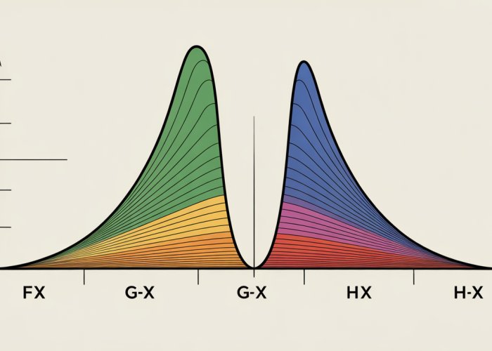
To visualize the Squeeze Theorem, we need a graph displaying three functions: g(x), f(x), and h(x).
The key condition is that g(x) ≤ f(x) ≤ h(x) over an open interval containing the point a (the limit point), possibly excluding a itself. This means that at any x-value within that interval, the value of f(x) always lies between the values of g(x) and h(x).

The graph should clearly label each function and the limit point a on the x-axis.
The y-axis will represent the function values.
Choose functions that visually demonstrate the "squeezing" effect effectively. For instance, consider f(x) = xsin(1/x) bounded by g(x) = -x² and h(x) = x².

Interpreting the Graph

The essence of the Squeeze Theorem becomes clear when we observe the behavior of the functions near the limit point a.
As x approaches a, both g(x) and h(x) approach the same limit L.
Because f(x) is trapped between g(x) and h(x), it is forced to also approach L.

Visually, this translates to the graphs of g(x) and h(x) "closing in" on f(x) as x gets closer to a.
The function f(x), unable to escape the narrowing gap, is effectively "squeezed" towards the same limit L.

The graph visually confirms that even if f(x) exhibits complex or oscillating behavior, its limit is still determined by the behavior of the bounding functions.

The Role of Graphing Tools

While hand-drawn sketches can be helpful for initial understanding, graphing software or online tools significantly enhance visualization.
Software like Desmos, GeoGebra, or Wolfram Alpha allows for precise plotting of functions, dynamic adjustments to parameters, and clearer observation of limit behavior.

These tools enable us to:

• Zoom in on the region near the limit point for detailed analysis.
• Experiment with different bounding functions to see how they affect the squeezing effect.
• Visualize the theorem with more complex functions that would be difficult to graph by hand.

By leveraging these resources, we can gain a more comprehensive understanding of the Squeeze Theorem and its applications. Visualizing the Squeeze Theorem through graphs provides an essential layer of understanding, making the abstract concept more concrete and accessible.

Applying the Squeeze Theorem: A Step-by-Step Example

The Squeeze Theorem shines when direct limit evaluation falters. Let’s dissect its application through a concrete example, providing a template for tackling similar problems.

We’ll evaluate the limit: lim (x→0) x²sin(1/x).

Identifying the Target and Bounding Functions

The first crucial step is recognizing when the Squeeze Theorem is appropriate. Observe that as x approaches 0, sin(1/x) oscillates wildly between -1 and 1.

Direct substitution leads to an indeterminate form, making standard techniques ineffective. This oscillatory behavior, combined with the bounding nature of sine, hints at the Squeeze Theorem’s applicability.

Our target function is therefore: f(x) = x²sin(1/x).

Now, we need to find two bounding functions, g(x) and h(x), such that g(x) ≤ f(x) ≤ h(x) for all x near 0 (excluding 0 itself).

Key Insight: The sine function is always bounded between -1 and 1.

Thus, -1 ≤ sin(1/x) ≤ 1.

Multiplying all parts of this inequality by x² (which is always non-negative) gives us: -x² ≤ x²sin(1/x) ≤ x².

Therefore, we can identify our bounding functions as:

• g(x) = -x²
• h(x) = x²

Rationale Behind the Choice of Bounding Functions

The selection of g(x) = -x² and h(x) = x² isn’t arbitrary. We leveraged the inherent boundedness of the sine function.

By multiplying this bounded inequality by x², we created functions that "squeeze" x²sin(1/x) as x approaches 0.

The x² term ensures that both bounding functions approach the same limit, a critical requirement for the Squeeze Theorem. This careful construction is the art of applying this theorem.

Evaluating the Limits of the Bounding Functions

The next step is to evaluate the limits of our bounding functions as x approaches 0:

lim (x→0) g(x) = lim (x→0) -x² = 0

lim (x→0) h(x) = lim (x→0) x² = 0

Both limits exist and are equal to 0. This satisfies another crucial condition of the Squeeze Theorem: the bounding functions must converge to the same limit.

Concluding with the Squeeze Theorem

Since -x² ≤ x²sin(1/x) ≤ x² for all x near 0 (excluding 0), and lim (x→0) -x² = lim (x→0) x² = 0, we can confidently apply the Squeeze Theorem.

The theorem states that if g(x) ≤ f(x) ≤ h(x) near a, and lim (x→a) g(x) = lim (x→a) h(x) = L, then lim (x→a) f(x) = L.

Therefore, we conclude that:

lim (x→0) x²sin(1/x) = 0.

Summarizing the Mathematical Steps

Let’s recap the mathematical journey:

1. Identify f(x): f(x) = x²sin(1/x)
2. Establish Bounds: -1 ≤ sin(1/x) ≤ 1
3. Multiply by x²: -x² ≤ x²sin(1/x) ≤ x²
4. Define g(x) and h(x): g(x) = -x², h(x) = x²
5. Evaluate Limits: lim (x→0) -x² = 0, lim (x→0) x² = 0
6. Apply Squeeze Theorem: lim (x→0) x²sin(1/x) = 0

By carefully identifying the target function, establishing the appropriate inequalities, and verifying the limit conditions, we successfully applied the Squeeze Theorem. This methodical approach is key to mastering this powerful limit evaluation technique.

That careful construction is the groundwork. But where else does the Squeeze Theorem commonly appear? As it turns out, trigonometric functions are a frequent and fertile ground for its application.

Squeeze Theorem and Trigonometric Functions

Trigonometric functions, with their oscillating and bounded behaviors, often present limits that are intractable by direct substitution or algebraic manipulation. This is where the Squeeze Theorem becomes an indispensable tool.

The Necessity of the Squeeze Theorem with Trigonometric Functions

Many limits involving trigonometric functions, especially those that result in indeterminate forms like 0/0, cannot be directly evaluated. The oscillatory nature of sine and cosine, and the asymptotic behavior of tangent and other related functions, complicate the limit-finding process.

Direct substitution often leads to expressions that are undefined or unhelpful, making the Squeeze Theorem a vital technique for navigating these challenges. The theorem’s ability to "sandwich" a troublesome function between two well-behaved functions allows us to determine its limit indirectly.

Examples with Sine, Cosine, and Tangent

The Squeeze Theorem can be applied across a range of trigonometric functions. While sine and cosine are the most common candidates due to their bounded nature (between -1 and 1), the theorem can be adapted to handle other trigonometric functions as well.

• Sine and Cosine: Problems like lim (x→0) x

  **sin(1/x) (discussed earlier) perfectly illustrate this.

  The sine function’s bounded nature is exploited to create a "squeeze" using simpler functions.

• Tangent: While less direct, the Squeeze Theorem can be used in conjunction with trigonometric identities to address limits involving tangent.

  For example, rewriting tangent in terms of sine and cosine can sometimes allow for strategic application of the theorem.

The Classic Example: lim (x→0) sin(x)/x

The limit lim (x→0) sin(x)/x is a cornerstone example in calculus, famous for its reliance on the Squeeze Theorem. Direct substitution yields the indeterminate form 0/0, rendering it unsolvable through elementary methods.

Geometric Proof of lim (x→0) sin(x)/x = 1

The proof typically involves a geometric construction within a unit circle. Consider a small angle x (in radians) in the first quadrant. We compare the areas of three regions: a triangle, a sector, and another triangle.

1. Area of Triangle 1 (smaller): (1/2)** base height = (1/2) 1

   **sin(x) = (1/2)sin(x).

2. Area of Sector: (1/2)** radius² angle = (1/2) 1²

   **x = (1/2)x.

3. Area of Triangle 2 (larger): (1/2)** base height = (1/2) 1 * tan(x) = (1/2)tan(x).

From the geometry, we observe that:

Area(Triangle 1) < Area(Sector) < Area(Triangle 2)

(1/2)sin(x) < (1/2)x < (1/2)tan(x)

Multiplying all parts by 2 and dividing by sin(x) (since sin(x) > 0 for small positive x):

1 < x/sin(x) < 1/cos(x)

Taking the reciprocal (and flipping the inequality signs):

cos(x) < sin(x)/x < 1

As x approaches 0, cos(x) approaches 1. Thus, we have:

lim (x→0) cos(x) = 1 and lim (x→0) 1 = 1

By the Squeeze Theorem, since sin(x)/x is "squeezed" between cos(x) and 1, both of which approach 1 as x approaches 0:

lim (x→0) sin(x)/x = 1

This result is fundamental and used extensively in evaluating other trigonometric limits. The geometric proof provides an intuitive understanding of why this limit holds true, solidifying the Squeeze Theorem’s power in resolving otherwise intractable problems.

That careful construction is the groundwork. But where else does the Squeeze Theorem commonly appear? As it turns out, trigonometric functions are a frequent and fertile ground for its application.

Common Mistakes and Pitfalls When Using the Squeeze Theorem

The Squeeze Theorem, while powerful, can be tricky to apply correctly. Recognizing and avoiding common pitfalls is crucial for mastering this technique and arriving at valid conclusions. Let’s explore some frequent errors encountered when employing the Squeeze Theorem.

Incorrectly Identifying Bounding Functions

One of the most common errors is selecting inappropriate bounding functions. The Squeeze Theorem hinges on the function in question being truly "sandwiched" between two others across an interval.

If the chosen functions do not consistently bound the target function, the theorem’s conditions are not met, and any resulting conclusion is invalid. Ensure that g(x) ≤ f(x) ≤ h(x) holds true for all x near the point of interest (except possibly at the point itself).

Failure to Verify Equal Limits

The Squeeze Theorem requires that the limits of both bounding functions, g(x) and h(x), must exist and be equal at the point in question.

A frequent mistake is finding bounding functions but neglecting to confirm that lim (x→a) g(x) = lim (x→a) h(x) = L.

If these limits are not equal, or if one or both do not exist, the Squeeze Theorem cannot be applied. This verification step is absolutely essential.

Misapplication of the Theorem

The Squeeze Theorem is not a universal limit-solving tool. It is specifically designed for situations where a function is bounded between two others.

Applying it when this condition isn’t met leads to incorrect results. For instance, if you can directly evaluate the limit using other techniques, the Squeeze Theorem might be unnecessary and even cumbersome. Always assess whether the theorem’s conditions are genuinely satisfied before attempting to use it.

Misinterpreting Inequality Signs

A seemingly minor, but critical error, involves misinterpreting or misusing the inequality signs. The order of the inequality is paramount.

If the inequality is reversed, i.e., g(x) ≥ f(x) ≥ h(x), the theorem’s logic is disrupted, and the conclusion becomes invalid. Double-check that your inequalities are correctly oriented and accurately reflect the relationships between the functions involved. Attention to detail in these inequalities is critical for a successful application of the Squeeze Theorem.

That careful construction is the groundwork. But where else does the Squeeze Theorem commonly appear? As it turns out, trigonometric functions are a frequent and fertile ground for its application.

Advanced Applications and Related Concepts

While the Squeeze Theorem shines in introductory calculus, its influence extends far beyond basic limit calculations. It forms a cornerstone in proving more complex limit theorems and finds application in real analysis. Exploring these advanced facets reveals the true power and versatility of this elegant mathematical tool.

Role in Proving Limit Theorems

The Squeeze Theorem isn’t just a problem-solving technique; it’s also a crucial component in establishing the validity of other significant limit theorems.

For example, it’s instrumental in proving the limit of sin(x)/x as x approaches 0, which then serves as a foundation for deriving derivatives of trigonometric functions.

Many proofs in calculus rely on the Squeeze Theorem to rigorously establish the existence and value of limits. Its logical structure provides a means to control a function’s behavior near a point, allowing mathematicians to build upon established results with confidence.

Connection to the Intermediate Value Theorem

The Intermediate Value Theorem (IVT) and the Squeeze Theorem might seem unrelated at first glance, but both deal with function behavior within a given interval. The IVT guarantees that if a continuous function takes on two values, it must also take on every value in between.

While the Squeeze Theorem doesn’t directly prove the IVT, understanding the concept of bounding functions, as used in the Squeeze Theorem, provides a valuable intuitive base.

The Squeeze Theorem reinforces the idea that function behavior can be constrained and predicted, which is a concept that resonates with the IVT’s focus on continuous functions taking on intermediate values. The difference, however, lies in their application: one deals with limits, the other with function values across an interval.

Squeeze Theorem in Real Analysis

Real analysis, the rigorous study of real numbers and functions, relies heavily on the Squeeze Theorem.

In this field, it is used to formally define concepts like continuity and convergence.

The precise nature of real analysis demands tools like the Squeeze Theorem, which provides a way to define limits and function behavior with mathematical certainty.

For instance, when dealing with sequences, the Squeeze Theorem can be used to determine convergence. If a sequence is bounded above and below by two sequences that converge to the same limit, the sequence in question must also converge to that limit.

This is particularly useful when direct methods of evaluating the limit are insufficient. The Squeeze Theorem provides a valuable alternative approach to establishing convergence rigorously.

Alright, now you’ve got the squeeze theorem limit down! Go forth and conquer those pesky limit problems. Hopefully, this made things a little easier. Best of luck!