Economics Supply Curve? What You Need To Know!

The law of supply, a fundamental principle influencing market behavior, directly shapes the economics supply curve. Producers, driven by profit motives, adjust their output based on price signals reflected in this curve. Supply-side economics leverages the understanding of the economics supply curve to influence macroeconomic policy. Changes in production costs are immediately visible, therefore shifting the economics supply curve and impacting market equilibrium.

In the realm of economics, supply is a foundational concept, representing the total amount of a specific good or service that is available to consumers.

It is the bedrock upon which producers make decisions about production levels, pricing strategies, and resource allocation.

Understanding the dynamics of supply is crucial for businesses, policymakers, and even individual consumers, as it influences everything from the price of groceries to the availability of the latest gadgets.

The Significance of the Supply Curve

At the heart of understanding supply lies the economics supply curve.

This curve is a visual representation of the relationship between the price of a good or service and the quantity that producers are willing to supply.

It provides invaluable insights into how market forces shape the availability of goods and services.

Understanding the supply curve helps businesses forecast production, optimize pricing, and respond strategically to changing market conditions.

For policymakers, it’s essential for crafting effective regulations and interventions that promote economic stability and growth.

Purpose of This Overview

This article aims to provide a comprehensive overview of the economics supply curve, demystifying its key concepts, applications, and implications.

We will explore the factors that influence the supply curve, examine its different types, and illustrate its role in determining market equilibrium.

Whether you are a student of economics, a business professional, or simply a curious observer of the economic landscape, this guide will equip you with the knowledge and tools to navigate the world of supply with confidence.

Defining the Supply Curve: Price and Quantity Relationship

Having established the foundational importance of understanding supply, we now turn our attention to defining the very tool that unlocks its secrets: the economics supply curve.

This curve isn’t just a line on a graph; it’s a visual representation of the intricate dance between price and quantity in the marketplace.

It is a relationship that dictates how much producers are willing to offer at various price points.

Unveiling the Economics Supply Curve

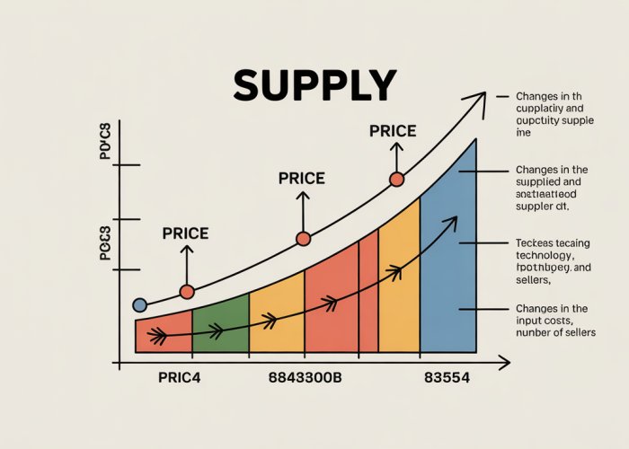
At its core, the economics supply curve illustrates the direct relationship between the price of a good or service and the quantity that producers are willing and able to supply to the market.

It plots price on the vertical axis (y-axis) and quantity on the horizontal axis (x-axis).

Each point on the curve represents a specific price-quantity combination, reflecting a producer’s willingness to supply a certain quantity at that given price.

The curve itself typically slopes upwards from left to right, illustrating a positive correlation between price and quantity.

The Law of Supply: The Driving Force

The upward slope of the supply curve is underpinned by the Law of Supply.

This fundamental economic principle states that, all other factors being equal, as the price of a good or service increases, the quantity supplied of that good or service will also generally increase.

Conversely, as the price decreases, the quantity supplied will generally decrease.

Why does this relationship hold?

Because higher prices incentivize producers to increase production, as they can earn greater profits.

Conversely, lower prices discourage production, as profits diminish.

Producers respond to price signals in the market, allocating resources to the production of goods and services that offer the highest potential returns.

The Law of Supply is the bedrock upon which the supply curve is built.

It offers invaluable insight into producer behavior and market dynamics.

The Supply Schedule: Data Behind the Curve

The supply schedule is a table that shows the exact quantity of a good or service that producers are willing to supply at different price points.

It provides the numerical data that is then used to construct the supply curve.

Imagine a table listing various prices for a product, alongside the corresponding quantities that a firm is prepared to offer at each price.

This table is the supply schedule.

The supply curve is simply a graphical representation of this data, making it easier to visualize the relationship between price and quantity.

The supply schedule is the foundation; the supply curve is the visual interpretation.

Together, they offer a comprehensive understanding of how producers respond to changing market conditions.

Having examined how the Law of Supply dictates the relationship between price and quantity, it’s crucial to acknowledge that price isn’t the only determinant of supply. The supply curve, while visually representing this price-quantity nexus, can shift its entire position in response to a multitude of other influencing factors. Understanding these non-price determinants is essential for a complete picture of supply dynamics.

Factors Shifting the Supply Curve: Beyond Price

While the supply curve illustrates the direct relationship between price and quantity supplied, it’s important to recognize that this relationship exists within a broader context. Several non-price factors can influence a producer’s willingness or ability to supply a good or service, causing the entire supply curve to shift. These factors are critical to understanding the complete picture of supply dynamics in any market.

Technology: The Efficiency Catalyst

Advancements in technology often lead to increased efficiency in production processes. New technologies can automate tasks, reduce waste, and optimize resource utilization.

These improvements lower the cost of production, allowing firms to supply more goods or services at any given price. This results in a rightward shift of the supply curve, indicating an increase in supply.

For example, the introduction of automated harvesting equipment in agriculture has significantly increased crop yields while reducing labor costs, thereby boosting the supply of agricultural products.

Input Prices: The Cost of Doing Business

Input prices, such as the cost of raw materials, labor, energy, and capital, play a crucial role in determining a firm’s cost of production.

An increase in input prices raises the cost of producing each unit, making it less profitable for firms to supply the same quantity at the same price.

Consequently, the supply curve shifts to the left, indicating a decrease in supply. Conversely, a decrease in input prices lowers production costs, leading to a rightward shift in the supply curve.

For instance, a rise in the price of crude oil, a key input for many industries, can increase the production costs for everything from plastics to transportation, ultimately reducing supply.

Government Regulations: The Regulatory Framework

Government regulations can also significantly impact supply. Regulations such as environmental laws, safety standards, and licensing requirements can impose additional costs on businesses.

More stringent regulations often increase the cost of compliance, leading to a decrease in supply and a leftward shift of the supply curve.

Conversely, deregulation or the removal of burdensome regulations can lower costs and increase supply, shifting the curve to the right.

For instance, strict environmental regulations on emissions from factories can increase the cost of production for manufacturers, leading to a decrease in the supply of certain goods.

Other Key Factors Influencing Supply

Beyond technology, input prices, and government regulations, several other factors can influence the supply of goods and services:

• Number of Sellers: A greater number of sellers in a market increases the overall supply, shifting the supply curve to the right. Conversely, a decrease in the number of sellers reduces supply, shifting the curve to the left.

• Future Expectations: Producers’ expectations about future prices and market conditions can also affect current supply decisions. If producers expect prices to rise in the future, they may reduce current supply to capitalize on higher future prices, shifting the supply curve to the left.

• Natural Disasters: Events like hurricanes, earthquakes, and floods can disrupt production processes and damage infrastructure, leading to a decrease in supply and a leftward shift of the supply curve. The severity and impact of natural disasters on supply often depend on the geographic location and the specific industries affected.

Having considered the factors that can shift the entire supply curve, it’s natural to ask how much supply changes in response to these shifts. The degree to which producers alter their output following a change in price, or in response to these other influences, is crucial for understanding market dynamics. This responsiveness is captured by the concept of elasticity of supply.

Elasticity of Supply: Measuring Responsiveness

Elasticity of supply measures the sensitivity of the quantity supplied of a good or service to a change in its price. In simpler terms, it tells us how much the quantity supplied will increase or decrease when the price goes up or down. This concept is vital for businesses making production and pricing decisions, and for policymakers forecasting market responses.

Understanding the Formula

Elasticity of supply is calculated as the percentage change in quantity supplied divided by the percentage change in price:

Elasticity of Supply = (% Change in Quantity Supplied) / (% Change in Price)

This formula yields a numerical value that indicates the degree of responsiveness. A higher value indicates a greater responsiveness to price changes, while a lower value indicates a lesser responsiveness.

Types of Supply Elasticity

The numerical value obtained from the elasticity of supply formula allows us to categorize supply into different types:

• Elastic Supply (Elasticity > 1): In this case, the percentage change in quantity supplied is greater than the percentage change in price. This means that producers are highly responsive to price changes. A small increase in price leads to a relatively large increase in quantity supplied, and vice versa.
  Products with readily available resources and flexible production processes tend to have elastic supply.

• Inelastic Supply (Elasticity < 1): Here, the percentage change in quantity supplied is less than the percentage change in price. Producers are not very responsive to price changes. Even if the price increases significantly, the quantity supplied only increases slightly.
  Products with limited resources, long production times, or high storage costs often exhibit inelastic supply.

• Unit Elastic Supply (Elasticity = 1): This is a special case where the percentage change in quantity supplied is exactly equal to the percentage change in price. For every 1% increase in price, the quantity supplied increases by 1%.

• Perfectly Elastic Supply (Elasticity = ∞): This theoretical extreme implies that producers are willing to supply any quantity at a given price, but none at any price below that. The supply curve is a horizontal line.

• Perfectly Inelastic Supply (Elasticity = 0): In this extreme, the quantity supplied is fixed, regardless of the price. The supply curve is a vertical line. For example, if there is only one original painting by a deceased artist, the supply is perfectly inelastic.

Factors Influencing Elasticity of Supply

Several factors determine the elasticity of supply for a particular good or service:

• Availability of Resources: If the resources needed to produce a good are readily available and easily obtainable, supply tends to be more elastic. If resources are scarce or difficult to acquire, supply will likely be inelastic.

• Production Time: Goods that can be produced quickly tend to have more elastic supply. If production takes a long time, supply is less elastic because producers cannot quickly respond to changes in price.

• Storage Capacity: If goods can be easily stored without significant cost or spoilage, producers can hold inventory and respond to price increases by releasing stored goods. This increases elasticity. Perishable goods with limited storage options tend to have inelastic supply.

• Spare Capacity: If firms have idle production capacity, they can quickly increase output in response to a price increase, resulting in more elastic supply. Firms operating at full capacity will find it difficult to increase production quickly, leading to inelastic supply.

• Ease of Entry and Exit: Industries with low barriers to entry allow new firms to enter the market quickly in response to higher prices, increasing supply elasticity. Conversely, industries with high barriers to exit may see firms continue to produce even when prices are low, resulting in lower elasticity.

• Time Horizon: Supply tends to be more elastic in the long run than in the short run. In the short run, firms may face constraints on their ability to increase production, such as fixed capital or limited access to resources. In the long run, firms have more flexibility to adjust their production processes and resource usage, making supply more responsive to price changes.

Understanding elasticity of supply is crucial for predicting how markets will respond to changes in price or other factors. Businesses can use this knowledge to make informed decisions about production, pricing, and inventory management, while policymakers can use it to forecast the impact of taxes, subsidies, and regulations on the economy.

Having considered the factors that can shift the entire supply curve, it’s natural to ask how much supply changes in response to these shifts. The degree to which producers alter their output following a change in price, or in response to these other influences, is crucial for understanding market dynamics. This responsiveness is captured by the concept of elasticity of supply. We now turn our attention to exploring the nuances of different types of supply curves, each offering a unique perspective on producer behavior.

Types of Supply Curves: Market, Individual, Short-Run, and Long-Run

Supply curves aren’t monolithic. They can be viewed from different angles, depending on the scope of analysis and the time horizon considered. Understanding these distinctions is critical for accurately interpreting market behavior. We’ll explore the contrasts between market and individual supply curves, as well as the important differences between short-run and long-run perspectives.

Market Supply Curve vs. Individual Supply Curve

The market supply curve represents the total quantity supplied of a good or service by all producers at various price levels. It’s essentially the horizontal summation of all individual supply curves in the market. This curve reflects the collective behavior of numerous firms.

The individual supply curve, on the other hand, depicts the quantity supplied by a single producer at different prices. This curve reflects the cost structure and production capacity of a specific firm. Understanding both is key for grasping market dynamics.

Aggregating to the Market Level

The market supply curve is derived by adding up the quantities that each individual firm is willing and able to supply at each given price.

For example, if at a price of $10, Firm A supplies 50 units and Firm B supplies 75 units, the market supply at $10 would be 125 units. This aggregation process is repeated for all possible prices.

Implications of the Distinction

The distinction between market and individual supply curves is crucial for analyzing market structure. In perfectly competitive markets, individual firms are small relative to the market. Therefore, their individual supply decisions have a negligible impact on the market price.

However, in markets with fewer producers (e.g., oligopolies), the supply decisions of individual firms can significantly influence market prices.

Short-Run Supply Curve vs. Long-Run Supply Curve

The time horizon plays a critical role in determining the shape and elasticity of the supply curve. We differentiate between short-run and long-run supply curves based on the flexibility firms have to adjust their production processes.

Short-Run Constraints

The short-run supply curve represents the quantity supplied by producers when at least one factor of production is fixed. This fixed factor often involves physical capital (e.g., factory size, machinery).

In the short run, firms can only adjust their output by changing the variable inputs. (e.g., labor, raw materials). This limited flexibility makes the short-run supply curve relatively inelastic, meaning quantity supplied is less responsive to price changes.

Long-Run Flexibility

The long-run supply curve represents the quantity supplied when all factors of production are variable. Firms have ample time to adjust their capital stock, enter or exit the industry, and adopt new technologies.

This greater flexibility makes the long-run supply curve generally more elastic than the short-run curve. Producers can respond more significantly to price changes over longer periods.

Industry Entry and Exit

A key factor differentiating the long run from the short run is the possibility of firms entering or exiting the industry. If prices rise, new firms may be attracted to enter, increasing market supply. Conversely, if prices fall, some firms may exit, reducing market supply. This entry and exit dynamic only occurs in the long run.

Implications for Market Outcomes

The elasticity of the supply curve in the short run versus the long run has significant implications for market outcomes. In the short run, a sudden increase in demand may lead to a sharp increase in price, as producers cannot quickly increase supply.

However, in the long run, the supply curve becomes more elastic. This allows producers to meet the increased demand with a smaller price increase, as they can adjust all factors of production.

Supply and Demand Equilibrium: Finding the Balance

Having considered the factors that can shift the entire supply curve, it’s natural to ask how much supply changes in response to these shifts. The degree to which producers alter their output following a change in price, or in response to these other influences, is crucial for understanding market dynamics. This responsiveness is captured by the concept of elasticity of supply. We now turn our attention to exploring the nuances of different types of supply curves, each offering a unique perspective on producer behavior. This understanding sets the stage for a crucial next step: examining how supply interacts with demand to establish equilibrium in the marketplace.

The Basics of Demand

Before diving into the interplay of supply and demand, it’s important to briefly establish the foundational concept of demand.

Demand, at its core, represents the consumer’s desire and ability to purchase a good or service at a given price.

Similar to the supply curve, the demand curve illustrates the relationship between price and quantity, but from the consumer’s perspective.

Typically, as the price of a good decreases, the quantity demanded increases, reflecting the Law of Demand.

This inverse relationship forms the basis for understanding consumer behavior in the market.

The Intersection: Supply, Demand, and Equilibrium

The magic truly happens when the supply and demand curves meet.

The market equilibrium is the point where the supply curve and the demand curve intersect.

At this point, the quantity supplied equals the quantity demanded, creating a balance in the market.

The price at this intersection is known as the equilibrium price, and the quantity is the equilibrium quantity.

This equilibrium represents a state of rest, where there is no inherent pressure for the price or quantity to change, assuming all other factors remain constant.

Surpluses, Shortages, and Price Adjustments

The market doesn’t always perfectly rest at equilibrium.

Disequilibrium occurs when the market price is either above or below the equilibrium price, leading to either a surplus or a shortage.

Understanding Surpluses

A surplus occurs when the market price is above the equilibrium price.

At this higher price, the quantity supplied exceeds the quantity demanded.

Producers are willing to supply more than consumers are willing to buy.

This excess supply creates downward pressure on the price, as sellers try to get rid of unsold inventory.

To eliminate the surplus, sellers will typically lower their prices, moving the market towards equilibrium.

Understanding Shortages

A shortage occurs when the market price is below the equilibrium price.

At this lower price, the quantity demanded exceeds the quantity supplied.

Consumers want to buy more than producers are willing to supply.

This excess demand creates upward pressure on the price, as consumers compete for limited goods.

Sellers, recognizing the high demand, will typically raise their prices, again moving the market towards equilibrium.

The Price Mechanism

The constant push and pull of surpluses and shortages are what drive the price mechanism in a market economy.

This mechanism ensures that prices adjust dynamically to reflect the underlying forces of supply and demand.

This continuous adjustment process helps to allocate resources efficiently, ensuring that goods and services are produced and consumed in quantities that best reflect consumer preferences and producer costs.

Real-World Examples: Applying the Supply Curve

The theoretical understanding of the supply curve gains practical relevance when viewed through the lens of real-world examples. Observing how different industries react to fluctuating production costs and technological shifts solidifies our grasp on this fundamental economic principle. Let’s delve into specific scenarios to illustrate the dynamic nature of supply in action.

The Agricultural Sector: Fertilizer Costs and Supply

Agriculture provides a compelling example of how changes in input costs directly affect supply. Fertilizer is a crucial input for many agricultural products, particularly crops.

The Impact of Increased Fertilizer Costs

When the cost of fertilizer rises, farmers face increased production expenses. This increase affects their profitability, which may influence supply decisions.

To illustrate, consider a scenario where the price of nitrogen-based fertilizer doubles due to geopolitical tensions affecting global supply chains. Farmers growing corn, wheat, and soybeans, heavily reliant on these fertilizers, now face substantially higher costs.

Supply Curve Shift

To mitigate losses, some farmers might reduce their planting acreage, opting for less fertilizer-intensive crops or leaving some land fallow. Others may continue planting at the same levels but are forced to increase the prices of their final product.

This collective behavior leads to a leftward shift in the supply curve for corn, wheat, and soybeans. At any given price point, the quantity supplied decreases, resulting in a lower equilibrium quantity and potentially higher market prices.

Long-Term Adjustments

Over time, farmers might explore alternative fertilizers, adopt more efficient application techniques, or invest in technologies that reduce fertilizer dependency. These long-term adjustments can partially offset the initial supply reduction, but the immediate impact of increased fertilizer costs is a clear demonstration of how input prices affect supply.

The Electronics Industry: Technological Innovation and Supply

The electronics industry provides a contrasting example where technological innovation dramatically influences supply. Consider the market for smartphones, laptops, and other consumer electronics.

The Role of Innovation

Rapid advancements in technology lead to increased efficiency in production, lower manufacturing costs, and the introduction of new and improved products. These advancements drive changes in the supply curve.

For example, the development of more efficient microchips or advanced manufacturing processes can significantly reduce the cost of producing smartphones. Companies can produce more units at a lower cost, increasing the quantity supplied at every price level.

Supply Curve Shift

This technological innovation results in a rightward shift of the supply curve. More smartphones are available at any given price, leading to a higher equilibrium quantity and potentially lower prices due to increased competition.

Moreover, innovation often leads to the creation of entirely new product categories, further expanding the overall supply of electronic gadgets. The introduction of wearable technology, such as smartwatches, illustrates this phenomenon.

Competition and Market Dynamics

As new technologies emerge and production costs decrease, more companies enter the market, increasing the overall supply and driving further innovation. This dynamic interplay between technology and supply is a hallmark of the electronics industry, where continuous improvement and market competition shape the landscape.

Alright, hopefully, you’ve got a better handle on the economics supply curve now. Go forth and analyze! Let us know what you think, and happy economics-ing!