Components of Force: Your Complete, Easy Guide (2024)

Understanding components of force is fundamental in physics, especially when analyzing situations involving inclined planes or projectile motion. Newton’s Laws of Motion provide the foundation for decomposing forces into perpendicular components, simplifying complex problems. These concepts are often explored using tools like free body diagrams, which visually represent all forces acting on an object. MIT OpenCourseWare offers accessible resources for anyone looking to deepen their understanding of vector resolution and the calculation of components of force. Using these fundamental concepts is how you can gain a complete understanding of complex force applications.

Force is a fundamental concept in physics, underpinning our understanding of how objects interact and move.

It’s not simply a push or a pull; it’s a more nuanced concept that requires careful consideration, especially when dealing with forces acting at angles.

The ability to dissect a force into its constituent parts, known as force components, is an indispensable skill for anyone venturing into the world of physics. This section will lay the groundwork for that skill.

Force as a Vector Quantity

At its core, force is a vector quantity. This means it possesses both magnitude (how strong the force is) and direction (where the force is pointing).

Think of pushing a box: the strength of your push is the magnitude, and the direction you’re pushing determines where the box will move.

Unlike scalar quantities, which are defined by magnitude alone (like temperature or mass), vectors require both pieces of information to be fully defined.

Understanding this vector nature is crucial because it dictates how we manipulate and analyze forces mathematically.

The Necessity of Resolving Forces into Components

Why can’t we just use the raw force value in calculations?

The challenge arises when forces act at angles to a chosen coordinate system (usually x and y axes).

Imagine pulling a sled diagonally; some of your force is pulling it forward, and some is lifting it upward. To accurately predict the sled’s motion, we need to know the exact contribution of each of these effects.

This is where the power of force components comes into play. By resolving a force into its x and y components, we essentially break it down into two forces that act parallel to our coordinate axes.

These components then allow us to analyze the effect of the force in each direction independently, greatly simplifying the overall problem.

Real-World Applications

Force component analysis isn’t just an abstract mathematical exercise; it’s a tool with widespread applications in the real world.

Consider the design of bridges: Engineers must carefully analyze the forces acting on the structure, including the weight of the bridge itself, the load of vehicles, and wind forces.

By resolving these forces into components, they can ensure the bridge is strong enough to withstand the various stresses and strains.

Another example lies in sports. A baseball player instinctively uses force components when throwing a ball at an angle to achieve maximum distance or accuracy. The angle of release directly affects the horizontal and vertical components of the force, and thus the trajectory of the ball.

From designing aircraft to understanding the biomechanics of human movement, force component analysis is an essential tool for engineers, scientists, and anyone seeking to understand the physical world around us.

Force is a fundamental concept in physics, underpinning our understanding of how objects interact and move.
It’s not simply a push or a pull; it’s a more nuanced concept that requires careful consideration, especially when dealing with forces acting at angles.
The ability to dissect a force into its constituent parts, known as force components, is an indispensable skill for anyone venturing into the world of physics. This section will lay the groundwork for that skill.
Force as a Vector Quantity
At its core, force is a vector quantity. This means it possesses both magnitude (how strong the force is) and direction (where the force is pointing).
Think of pushing a box: the strength of your push is the magnitude, and the direction you’re pushing determines where the box will move.
Unlike scalar quantities, which are defined by magnitude alone (like temperature or mass), vectors require both pieces of information to be fully defined.
Understanding this vector nature is crucial because it dictates how we manipulate and analyze forces mathematically.
The Necessity of Resolving Forces into Components
Why can’t we just use the raw force value in calculations?
The challenge arises when forces act at angles to a chosen coordinate system (usually x and y axes).
Imagine pulling a sled diagonally; some of your force is pulling it forward, and some is lifting it upward. To accurately predict the sled’s motion, we need to know the exact contribution of each of these effects.
This is where the power of force components comes into play, allowing us to break down complex forces into manageable, perpendicular parts.

Force, Vectors, and Scalars: Laying the Foundation

Before delving into the intricacies of force components, it’s essential to establish a solid foundation in the fundamental concepts that govern their behavior. We must clearly define force, vectors, and scalars, and understand how they relate to each other. This will provide the necessary framework for comprehending the nature of force and how it is mathematically represented.

Defining Force: The Agent of Change

At its most basic, force is an interaction that, when unopposed, will alter the motion of an object. This alteration can take the form of a change in velocity (acceleration), a change in direction, or both. It’s the "push" or "pull" that causes an object to speed up, slow down, or change direction.

Consider a stationary ball: it remains at rest until a force, such as a kick, acts upon it. Similarly, a moving car maintains its velocity until a force, like the brakes, causes it to decelerate. This ability to initiate or modify motion is what defines force.

Vectors: Quantities with Direction and Magnitude

Vectors are quantities that are fully described by both their magnitude and direction. The magnitude represents the size or strength of the quantity, while the direction indicates the way it is oriented in space.

Examples of Vectors

Common examples of vector quantities include:

• Velocity: The rate at which an object changes position, along with the direction of movement (e.g., 20 m/s east).
• Displacement: The change in position of an object from its starting point, also including direction (e.g., 10 meters north).
• Acceleration: The rate at which an object changes its velocity, also with a specific direction (e.g., 5 m/s² downwards).

These examples illustrate how direction is an integral part of a vector quantity’s definition. Removing the directional component would leave the quantity incomplete.

Scalars: Quantities Defined by Magnitude Alone

In contrast to vectors, scalars are quantities that are completely defined by their magnitude alone. Direction is irrelevant for scalar quantities.

Examples of Scalars

Some familiar examples of scalar quantities include:

• Mass: A measure of an object’s inertia, or resistance to acceleration (e.g., 5 kg).
• Time: A measure of duration (e.g., 10 seconds).
• Temperature: A measure of the average kinetic energy of the particles in a substance (e.g., 25 degrees Celsius).
• Speed: The rate at which an object covers distance, regardless of direction (e.g., 30 m/s).

Notice that these quantities are fully defined by their numerical value and unit of measurement. Direction plays no role in their definition.

Forces as Vectors: Representing Magnitude and Direction

Forces, being vector quantities, are represented mathematically as vectors. This means that when we describe a force, we must specify both how strong it is (magnitude) and in what direction it is acting.

Typically, forces are visualized using arrows. The length of the arrow corresponds to the magnitude of the force: a longer arrow represents a stronger force, while the direction the arrow points indicates the direction of the force.

For instance, a force of 10 Newtons pushing an object to the right would be represented by an arrow of a certain length pointing horizontally to the right. A force of 5 Newtons pulling an object upwards would be represented by a shorter arrow pointing vertically upwards.

This visual representation is crucial for understanding how forces interact and combine, setting the stage for more complex analysis. By treating forces as vectors, we gain the ability to use mathematical tools to predict and explain the motion of objects.

Trigonometry: The Mathematical Toolkit

The ability to break down forces into manageable components hinges on a critical mathematical discipline: trigonometry. While force vectors provide a visual representation of magnitude and direction, trigonometry provides the precise tools needed to quantify those aspects. Without a firm grasp of trigonometric principles, particularly the sine and cosine functions, accurately resolving forces becomes a significantly more challenging task.

Sine and Cosine: Unlocking Force Components

Trigonometric functions, specifically sine (sin) and cosine (cos), are essential tools for dissecting a force vector into its x and y components. These functions provide a well-defined relationship between an angle within a right triangle and the ratio of its sides. This relationship is the cornerstone of force resolution.

Understanding how these functions work within the context of a right triangle is paramount.

• Sine (sin θ): Represents the ratio of the length of the side opposite the angle θ to the length of the hypotenuse.

• Cosine (cos θ): Represents the ratio of the length of the side adjacent to the angle θ to the length of the hypotenuse.

In force analysis, the hypotenuse corresponds to the magnitude of the force vector itself. The angle (θ) is the angle between the force vector and a chosen reference axis, typically the x-axis. Therefore, the x and y components of the force can be determined using these trigonometric relationships.

Deriving Force Components with Trigonometry

The x and y components of a force vector represent the influence of that force along the horizontal and vertical axes, respectively. Using trigonometric functions, we can calculate these components with accuracy. The x-component (Fx) corresponds to the horizontal influence, while the y-component (Fy) corresponds to the vertical influence.

Calculating the X-Component

The x-component of a force vector is calculated using the cosine function:

Fx = F

**cos(θ)

Here, ‘F’ represents the magnitude of the force vector, and ‘θ’ is the angle between the force vector and the x-axis. The cosine of the angle gives us the ratio of the adjacent side (Fx) to the hypotenuse (F).

Calculating the Y-Component

Similarly, the y-component of a force vector is calculated using the sine function:

Fy = F** sin(θ)

In this case, the sine of the angle gives us the ratio of the opposite side (Fy) to the hypotenuse (F). This calculation provides the magnitude of the force acting along the y-axis.

Visualizing the Application of Sine and Cosine

Imagine a force vector acting at an angle θ to the x-axis. By drawing a vertical line from the tip of the force vector to the x-axis, we create a right triangle. The force vector itself becomes the hypotenuse of this triangle.

The length of the base of the triangle represents the x-component (Fx), and the length of the height represents the y-component (Fy). The angle θ is the angle between the force vector and the x-axis.

Therefore, visualizing this right triangle helps to understand how sine and cosine functions are used to determine the magnitudes of Fx and Fy, effectively resolving the force vector into its constituent parts. This process transforms a single angled force into two perpendicular forces, simplifying subsequent calculations and analysis.

Sine and cosine equip us with the ability to extract the x and y components of force, but their application relies on a clear definition of the force vector itself. This definition hinges on two fundamental properties: its magnitude and its angle relative to a chosen reference. Together, magnitude and direction paint a complete picture of the force and allow us to perform meaningful calculations.

Angles and Magnitude: Defining the Force Vector

The force vector is fully defined by its magnitude (strength) and its angle (direction). Understanding these two properties is paramount for accurate force analysis. Let’s delve deeper into each aspect.

Magnitude: The Strength of the Force

The magnitude of a force vector, often denoted as |F| or simply F, represents the intensity or strength of the force. It’s a scalar quantity, expressed in units like Newtons (N) in the SI system or pounds (lbs) in the imperial system. A larger magnitude indicates a greater "push" or "pull."

For example, a force of 100 N has twice the "pushing power" of a 50 N force. The magnitude is always a positive value, as it represents the absolute size of the force.

Angle: Specifying Direction

The angle, typically represented by the Greek letter theta (θ), specifies the direction of the force vector relative to a chosen reference axis. This axis is usually the positive x-axis in a standard Cartesian coordinate system. The angle is measured in degrees or radians, with counter-clockwise rotation from the reference axis considered positive.

The angle dictates how much of the force acts horizontally and vertically. An angle of 0° indicates a force acting purely along the x-axis, while an angle of 90° indicates a force acting purely along the y-axis.

The Interplay of Angle and Magnitude

The magic happens when we combine magnitude and angle. Different combinations yield vastly different force components. A large magnitude at a shallow angle will result in a large horizontal component and a small vertical component. Conversely, a small magnitude at a steep angle will result in a small horizontal component and a large vertical component.

Consider these examples:

• Example 1: A force of 50 N acting at an angle of 30° relative to the x-axis. This force will have a significant horizontal component and a smaller vertical component.
• Example 2: A force of 20 N acting at an angle of 60° relative to the x-axis. This force, despite having a smaller magnitude than Example 1, may have a similar or even larger vertical component.

This underscores the importance of considering both magnitude and angle when analyzing forces.

Visualizing Force Vectors

Diagrams are invaluable for visualizing force vectors and their components. Each force is represented as an arrow, with the length of the arrow proportional to the magnitude of the force. The direction of the arrow represents the angle.

Consider a diagram with the following:

• A force vector of magnitude 10 N at an angle of 45°.
• A force vector of magnitude 15 N at an angle of 135°.
• A force vector of magnitude 5 N at an angle of 270°.

By visually inspecting the diagram, one can qualitatively assess the relative sizes of the x and y components for each force. The 10 N force at 45° will have roughly equal x and y components. The 15 N force at 135° will have a negative x component and a positive y component. The 5 N force at 270° will have no x component and a negative y component.

These diagrams help bridge the gap between abstract mathematical concepts and intuitive understanding. They provide a visual aid for predicting how forces will affect the motion of an object.

Angles and magnitude work together to fully define a force vector. But what happens when we need to work with that force in a practical problem? That’s where resolving forces into their components comes in, allowing us to analyze forces in a way that aligns with our chosen coordinate system.

Resolution of Forces: Breaking it Down

The process of resolving forces involves breaking down a single force vector into its x and y components.

This is a crucial skill in physics.

It simplifies complex problems.

By understanding how to decompose a force, we can analyze its effect in specific directions. This helps us to more accurately predict its impact on an object’s motion or equilibrium.

The Goal: Finding x and y Components

The primary goal of resolving a force is to determine its x-component (Fx) and its y-component (Fy).

These components represent the effective force acting along the x-axis and the y-axis, respectively.

Instead of dealing with a single force acting at an angle, we can analyze the effects of two forces acting perpendicularly.

This simplification makes problem-solving significantly easier.

Step-by-Step Guide: Calculating Components with Trigonometry

Trigonometry is our essential tool for resolving forces.

Here’s a step-by-step guide:

1. Identify the Force Vector:
   Determine the magnitude (F) of the force and its angle (θ) relative to the positive x-axis.

2. Calculate the x-Component (Fx):
   Use the following formula:

   • Fx = F cos(θ)

     **

   The cosine function relates the angle to the adjacent side of a right triangle, which in this case is the x-component.

3. Calculate the y-Component (Fy):
   Use the following formula:

   • Fy = F sin(θ)**

   The sine function relates the angle to the opposite side of a right triangle, which in this case is the y-component.

4. Express the Force in Component Form:
   Represent the force as a sum of its components:

   • F = Fxi + Fyj, where i and j are the unit vectors in the x and y

     **directions, respectively.

Example

Imagine a force of 50 N acting at an angle of 30° relative to the x-axis.

Let’s calculate its x and y components:

• Fx = 50 N** cos(30°) ≈ 43.3 N
• Fy = 50 N * sin(30°) = 25 N

This means the force has an effective "push" of 43.3 N in the x direction and 25 N in the y direction.

Visualizing the Resolution Process

Diagrams are invaluable when resolving forces.

A typical diagram will show:

• The original force vector F as an arrow originating from a point.
• The x-axis and y-axis forming a Cartesian coordinate system.
• The angle θ between the force vector and the x-axis.
• The x-component Fx as an arrow along the x-axis.
• The y-component Fy as an arrow along the y-axis.

The x and y components form the legs of a right triangle, with the original force vector as the hypotenuse.
This visual representation reinforces the relationship between the force, its components, and the trigonometric functions used to calculate them.

By understanding and applying the process of force resolution, you can simplify complex force problems and gain deeper insights into the behavior of objects under the influence of multiple forces.

Angles and magnitude work together to fully define a force vector. But what happens when we need to work with that force in a practical problem? That’s where resolving forces into their components comes in, allowing us to analyze forces in a way that aligns with our chosen coordinate system. It’s not simply about blindly applying formulas, but rather about strategically setting up your problem for success.

Coordinate Systems: Choosing the Right Frame of Reference

The choice of coordinate system is paramount when dissecting forces into manageable components. It is your lens, shaping how you perceive and calculate these components. A poorly chosen system can unnecessarily complicate the problem, while a well-chosen one can dramatically simplify it.

The essence of choosing wisely lies in aligning the coordinate axes with the dominant directions of the forces or motion involved.

The Standard Cartesian Coordinate System

The familiar Cartesian coordinate system, with its perpendicular x-axis and y-axis, forms the bedrock of many force analyses. Convention dictates that the x-axis is horizontal and the y-axis is vertical, creating a natural framework for describing horizontal and vertical motion.

This system is intuitive for scenarios where forces predominantly act along these axes, such as objects moving on a flat surface or forces aligned with gravity. It provides a clear and straightforward way to resolve forces into their components.

The Power of Rotation: Simplifying Analysis

While the standard Cartesian system is a reliable starting point, it’s not always the optimal choice. In certain situations, rotating the coordinate system can significantly simplify the problem.

Consider an object resting on an inclined plane. Instead of using the standard vertical/horizontal axes, we can rotate our coordinate system so that the x-axis aligns with the slope of the plane and the y-axis is perpendicular to it.

This rotation elegantly transforms the problem: the normal force and the frictional force now lie entirely along the axes, requiring no further resolution. Only the gravitational force needs to be resolved into components parallel and perpendicular to the plane.

This strategic alignment drastically reduces the number of calculations and minimizes the chances of error.

Knowing When to Rotate

So, how do you know when a rotation is beneficial? Look for situations where a dominant force or direction of motion is at an angle to the standard axes. Inclined planes are the quintessential example.

However, this principle extends to any scenario where aligning an axis with a key direction streamlines the force analysis.

The Impact of Orientation on Force Component Signs

The orientation of your coordinate system directly affects the signs (+ or -) of the force components. This is crucial because the signs indicate the direction of the force component along the respective axis.

In the standard Cartesian system, forces acting to the right along the x-axis are positive, while forces acting to the left are negative. Similarly, upward forces along the y-axis are positive, and downward forces are negative.

When you rotate the coordinate system, these sign conventions shift accordingly. For example, if you rotate the axes by 90 degrees clockwise, what was initially a positive y-component now becomes a positive x-component.

Navigating Sign Conventions

Carefully consider the orientation of your axes and the direction of each force component relative to those axes. A clear understanding of these sign conventions is essential for correctly applying Newton’s laws of motion and achieving accurate results. Always double-check the signs of your components to ensure they align with the physical situation you’re analyzing.

Resultant Force: Unifying Multiple Forces into One

Angles and magnitude work together to fully define a force vector. But what happens when we need to work with that force in a practical problem? That’s where resolving forces into their components comes in, allowing us to analyze forces in a way that aligns with our chosen coordinate system. It’s not simply about blindly applying formulas, but rather about strategically setting up your problem for success.

Now, imagine a scenario where an object is subjected to not one, but multiple forces acting simultaneously. How do we determine the overall effect of these forces? This is where the concept of resultant force becomes indispensable.

The resultant force, also known as the net force, is the single force that encapsulates the combined effect of all individual forces acting on an object. Understanding how to calculate the resultant force is critical for predicting an object’s motion and analyzing its equilibrium.

Understanding the Resultant Force

Think of the resultant force as the "summary" of all the forces acting on an object. It represents the net push or pull experienced by the object, dictating whether it will accelerate, decelerate, or remain stationary.

If the resultant force is zero, the object is in equilibrium. This doesn’t necessarily mean the object is at rest; it could be moving at a constant velocity.

Vector Addition: The Key to Finding the Resultant

Since forces are vectors, we can’t simply add their magnitudes together. We need to consider both their magnitudes and directions. This is where vector addition comes into play.

The most common and effective method for vector addition involves breaking down each force into its x and y components.

Breaking Down the Process

1. Resolve Each Force: For each individual force acting on the object, determine its x and y components (Fx and Fy) using trigonometric functions (sine and cosine) as discussed earlier. Remember to pay attention to the signs of the components based on the quadrant in which the force vector lies.

2. Sum the Components: Add all the x-components together to find the x-component of the resultant force (Rx). Similarly, add all the y-components together to find the y-component of the resultant force (Ry).

   Rx = F1x + F2x + F3x + …

   Ry = F1y + F2y + F3y + …

3. Reconstruct the Resultant: Now that you have Rx and Ry, you can determine the magnitude and direction of the resultant force.

Finding Magnitude and Direction

With the x and y components of the resultant force in hand, we can use the Pythagorean theorem to find its magnitude:

R = √(Rx² + Ry²)

This gives you the strength of the overall force acting on the object.

To find the direction (angle θ) of the resultant force, we use the inverse tangent function:

θ = tan⁻¹(Ry / Rx)

Important Note: The arctangent function (tan⁻¹) only gives angles in the range of -90° to +90°. You may need to adjust the angle based on the signs of Rx and Ry to ensure it falls in the correct quadrant. Consider the following:

• If Rx is positive: the angle is in the 1st or 4th quadrant.
• If Rx is negative: the angle is in the 2nd or 3rd quadrant.

The Power of Resultant Force

Understanding how to calculate the resultant force is a fundamental skill in physics and engineering. It allows us to predict the motion of objects under the influence of multiple forces, design structures that can withstand various loads, and analyze complex systems where forces interact in intricate ways. Mastering this concept opens the door to a deeper understanding of the physical world around us.

Vector addition provides a powerful method for determining the resultant force from individual force components. But, to truly master force analysis, we need a visual tool that allows us to organize and understand all the forces acting on an object simultaneously. This is where free body diagrams come into play.

Free Body Diagrams: Visualizing Forces and Their Components

A free body diagram (FBD) is a simplified representation of an object and the external forces acting upon it.

It isolates the object of interest from its surroundings, allowing us to focus solely on the forces that directly influence its motion.

The FBD serves as a visual aid for applying Newton’s Laws of Motion and solving for unknown forces.

The Purpose of Free Body Diagrams

The primary goal of an FBD is to provide a clear and concise representation of all forces acting on an object.

This visual representation allows us to:

• Identify all relevant forces.
• Determine their directions.
• Resolve forces into components.
• Apply Newton’s Laws of Motion accurately.

By systematically constructing an FBD, we can avoid overlooking crucial forces and ensure that our analysis is complete and accurate.

Constructing a Free Body Diagram: A Step-by-Step Guide

Creating an effective free body diagram involves a series of steps, each contributing to the clarity and accuracy of the final representation.

Step 1: Represent the Object as a Point Mass

The first step in creating an FBD is to represent the object of interest as a simple point mass.

This simplification allows us to focus on the forces acting on the object without being distracted by its shape or size.

The location of the point mass is not critical, but it’s generally placed at the object’s center of mass.

Step 2: Identify and Draw External Forces

Next, identify all external forces acting on the object.

These forces can include:

• Weight (W): The force of gravity acting on the object, always directed downward.
• Normal Force (N): The force exerted by a surface perpendicular to the object in contact.
• Tension (T): The force exerted by a string, rope, or cable, always directed along the direction of the string.
• Applied Force (F): A force exerted by a person or another object.
• Friction (f): A force that opposes motion, directed parallel to the surface of contact.

Draw each force as an arrow originating from the point mass, with the length of the arrow representing the magnitude of the force and the direction of the arrow indicating the force’s direction.

Step 3: Label Each Force with its Magnitude and Direction

Clearly label each force arrow with its magnitude and direction.

Use appropriate symbols to represent the forces (e.g., W for weight, N for normal force, T for tension).

Indicate the angle of each force with respect to a reference axis (usually the x-axis).

This labeling ensures that all relevant information is readily available for subsequent calculations.

Step 4: Resolve Forces into X and Y Components

If any forces are acting at an angle to the coordinate axes, resolve them into their x and y components.

This involves using trigonometric functions (sine and cosine) to determine the magnitudes of the component forces.

Represent the components as arrows along the x and y axes, originating from the point mass.

Label each component with its magnitude and direction (e.g., Fx = Fcos(θ), Fy = Fsin(θ)).

Applying Free Body Diagrams to Newton’s Laws of Motion

Once the free body diagram is complete, it can be used to apply Newton’s Laws of Motion.

Recall Newton’s First Law, which states that an object at rest stays at rest and an object in motion stays in motion with the same speed and in the same direction unless acted upon by a net force.

Newton’s Second Law provides the mathematical relationship between force, mass, and acceleration: ΣF = ma, where ΣF is the vector sum of all forces acting on the object, m is the mass of the object, and a is the acceleration of the object.

Newton’s Third Law states that for every action, there is an equal and opposite reaction.

By applying Newton’s Second Law to the x and y components of the forces in the FBD, we can obtain a set of equations that can be solved for unknown quantities, such as acceleration, tension, or normal force.

For example, if an object is in equilibrium (i.e., not accelerating), the sum of the forces in both the x and y directions must be zero (ΣFx = 0, ΣFy = 0).

Vector addition provides a powerful method for determining the resultant force from individual force components. But, to truly master force analysis, we need a visual tool that allows us to organize and understand all the forces acting on an object simultaneously. This is where free body diagrams come into play.

Equilibrium: When Forces Balance

Understanding the conditions under which forces balance is paramount to grasping the fundamental principles of statics and dynamics. Equilibrium, in its essence, represents a state of balance, where the net effect of all forces acting on an object results in no acceleration. This concept is critical in numerous engineering and physics applications, from designing stable structures to analyzing the motion of objects.

Defining Equilibrium

Equilibrium is defined as a state in which the net force acting on an object is zero. This means that the vector sum of all forces, when resolved into their components, must equal zero in every direction. In simpler terms, the forces pushing or pulling an object to the right must be exactly balanced by the forces pushing or pulling it to the left. Similarly, upward and downward forces must also be balanced.

Mathematically, we can express this condition as:

∑F = 0

Where ∑F represents the vector sum of all forces acting on the object.

Static vs. Dynamic Equilibrium

It’s crucial to differentiate between two types of equilibrium: static and dynamic. Static equilibrium refers to a scenario where the object is at rest. Think of a book sitting on a table. The forces acting on it (gravity downwards and the normal force from the table upwards) are balanced, and the book remains motionless.

Dynamic equilibrium, on the other hand, occurs when an object is moving at a constant velocity. In this case, while the object is in motion, its velocity isn’t changing, implying zero acceleration. A car moving down a straight highway at a steady speed is a good example. The driving force provided by the engine counters the opposing forces of air resistance and friction, resulting in constant velocity and dynamic equilibrium.

Applying Equilibrium Conditions

The power of understanding equilibrium lies in its ability to solve for unknown forces. Since the net force in each direction must be zero, we can establish equations by summing the force components along the x and y axes.

These equations are:

∑Fx = 0
∑Fy = 0

Where ∑Fx is the sum of all force components in the x-direction, and ∑Fy is the sum of all force components in the y-direction.

By applying these equilibrium conditions to a free body diagram of an object, we can create a system of equations that can be solved to find the magnitude and direction of unknown forces. For example, if we know all but one of the forces acting on a stationary object, we can use these equations to determine the unknown force required to maintain equilibrium.

This concept is pivotal in structural engineering, where ensuring buildings and bridges remain in static equilibrium is paramount to safety. The same principles extend to dynamic systems as well, allowing engineers and scientists to analyze and predict the behavior of moving objects under various force conditions. Understanding equilibrium is therefore not merely an academic exercise, but a critical tool for real-world applications.

Equilibrium, in its essence, highlights the point where all forces acting on an object balance each other out, creating a net force of zero and thereby preventing any acceleration. Now that we have defined the concept of equilibrium, it is helpful to see how this plays out in real-world scenarios, particularly in the presence of applied forces and the ever-present force of friction.

Applied Force and Friction: Real-World Examples

Force components are not abstract mathematical constructs; they are essential for understanding and predicting the behavior of objects in everyday situations. When we analyze forces acting on an object, understanding the role of applied forces and friction becomes paramount.

Understanding Applied Force

Applied force is simply the force exerted on an object by an external agent, such as a person pushing a box, a car towing another vehicle, or a motor lifting an elevator.

It’s the force that initiates or alters the motion of an object.

Analyzing applied force involves determining its magnitude and direction. These factors will consequently allow us to resolve the force into its components.

For example, consider pushing a lawnmower: the force you exert has both a horizontal component (moving the mower forward) and a vertical component (potentially lifting the mower slightly, reducing its contact with the ground).

The Opposing Force: Friction

Friction is a force that opposes motion between surfaces in contact.

It’s crucial in many real-world scenarios, sometimes desirable (allowing us to walk or drive) and other times undesirable (causing wear and energy loss in machines).

Types of Friction

Static friction prevents an object from moving when a force is applied, while kinetic friction opposes the motion of an object already in motion.

The magnitude of frictional force depends on the nature of the surfaces in contact and the normal force (the force pressing the surfaces together).

Resolving Friction into Components

Like any force, friction can be resolved into components. Consider a block sliding down an inclined plane.

The frictional force acts parallel to the surface, opposing the motion.

In this scenario, we often resolve the gravitational force acting on the block into components parallel and perpendicular to the plane. The frictional force directly opposes the parallel component of gravity.

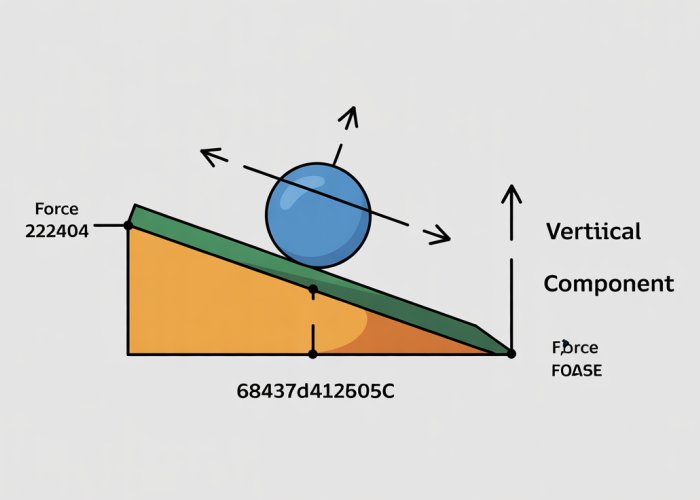
The Inclined Plane: A Classic Example

One of the most illustrative examples of force component analysis is the inclined plane problem.

Imagine a block resting on a ramp. Gravity pulls the block downwards, but the ramp prevents it from falling straight down.

Forces at Play

The weight of the block (force due to gravity) can be resolved into two components:

• One component perpendicular to the ramp (Fn = mg

  **cosθ), which is balanced by the normal force exerted by the ramp.

• Another component parallel to the ramp (Fp = mg**sinθ), which tends to pull the block down the incline.

Here, m is the mass of the block, g is the acceleration due to gravity, and θ is the angle of inclination of the ramp.

Introducing Friction to the Mix

Now, let’s add friction.

As the block tends to slide down the ramp, friction opposes this motion with a force (Ff) acting up the ramp.

If the block is at rest, static friction equals the parallel component of gravity, preventing the block from sliding.

If the block is sliding, kinetic friction opposes the motion.

The magnitude of kinetic friction is given by Ff = μk

**Fn, where μk is the coefficient of kinetic friction.

Calculating the Net Force

The net force acting on the block along the inclined plane is the difference between the parallel component of gravity and the frictional force:

Fnet = Fp – Ff = mg**sinθ – μk mgcosθ

If the net force is positive, the block accelerates down the ramp. If it’s zero, the block slides down at a constant velocity (dynamic equilibrium). If the static friction is greater than the parallel component of gravity, the block remains at rest (static equilibrium).

A Numerical Example

Let’s say we have a 5 kg block on a ramp inclined at 30 degrees, with a coefficient of kinetic friction of 0.2.

We can calculate the forces acting on the block:

• Fn = 5 kg 9.8 m/s² cos(30°) ≈ 42.4 N
• Fp = 5 kg 9.8 m/s² sin(30°) = 24.5 N
• Ff = 0.2 * 42.4 N ≈ 8.5 N
• Fnet = 24.5 N – 8.5 N = 16 N

The net force is positive, so the block accelerates down the ramp. We can further calculate the acceleration using Newton’s second law (F = ma):

a = Fnet / m = 16 N / 5 kg = 3.2 m/s²

Real-World Implications

Understanding these concepts is vital in various fields. Engineers use them to design safe bridges and buildings, taking into account the forces of gravity, wind, and the materials’ properties.

Physicists use them to study the motion of objects, from projectiles to planets.

Newton’s Laws of Motion: Applying Force Components to Dynamics

Having understood how to dissect forces into components and represent them visually, the next step is to use these tools within the framework of Newton’s Laws of Motion to analyze dynamic systems.

Newton’s Laws provide the fundamental rules governing the relationship between forces and motion, and mastering their application is essential for solving a wide range of physics problems.

A Concise Review of Newton’s Laws

Before delving into the application of force components, it’s helpful to have a quick review of Newton’s Laws of Motion:

• Newton’s First Law (Law of Inertia): An object at rest stays at rest, and an object in motion stays in motion with the same speed and in the same direction unless acted upon by a force.

  This law establishes the concept of inertia, the tendency of an object to resist changes in its state of motion.

• Newton’s Second Law: The acceleration of an object is directly proportional to the net force acting on the object, is in the same direction as the net force, and is inversely proportional to the mass of the object.

  Mathematically, this is expressed as F = ma, where F is the net force, m is the mass, and a is the acceleration.
  Newton’s Second Law is the cornerstone of dynamics calculations.

• Newton’s Third Law: For every action, there is an equal and opposite reaction.

  This law states that forces always occur in pairs.
  When one object exerts a force on another, the second object exerts an equal and opposite force back on the first.

Force Components and Newton’s Second Law: The Key Connection

The true power of force component analysis becomes apparent when applying Newton’s Second Law. When multiple forces act on an object at various angles, directly summing the forces is not possible. This is where resolving forces into components becomes essential.

1. Free Body Diagram (FBD): As we discussed, start by drawing a free body diagram, representing all forces acting on the object.

2. Resolve Forces: Resolve each force into its x and y components, aligning with the chosen coordinate system.

3. Net Force Calculation: Calculate the net force in each direction by summing the components:

   • F

     _net,x = F1x + F2x + F3x + …

   • F_net,y = F1y + F2y + F3y + …

4. Apply Newton’s Second Law: Apply Newton’s Second Law separately in each direction:

   • Fnet,x = m

     **ax

   • Fnet,y = m** ay

5. Solve for Acceleration: Solve the resulting equations for the acceleration components, ax and ay.
   The components fully describe the object’s acceleration.

By using this approach, a complex problem involving multiple forces at angles is simplified into two separate, easier-to-solve equations.

Examples of Newton’s Laws with Force Components

Example 1: Block on an Inclined Plane

Consider a block of mass m sliding down an inclined plane with an angle θ, with some friction force f opposing motion. To find the acceleration:

1. Draw a FBD: Include weight (mg), normal force (N), and friction (f).

2. Resolve Forces: Resolve weight into components parallel (mgsin(θ)) and perpendicular (mgcos(θ)) to the plane.

3. Apply Newton’s Second Law:
   Along the plane: mgsin(θ) – f = ma
   Perpendicular to the plane: N – mg*cos(θ) = 0 (no acceleration in this direction)

4. Solve for Acceleration: Solve for a.

Example 2: Object Suspended by Two Cables

An object is suspended by two cables at different angles. To determine the tension in each cable:

1. Draw a FBD: Include tensions T1 and T2 in the cables, and the weight of the object (mg).

2. Resolve Forces: Resolve T1 and T2 into x and y components based on their angles.

3. Apply Newton’s Second Law (Equilibrium):
   Horizontal: T1x – T2x = 0 (no acceleration in this direction)
   Vertical: T1y + T2y – mg = 0 (no acceleration in this direction)

4. Solve for Tensions: Solve the system of equations to find T1 and T2.

These examples illustrate how breaking down forces into components and applying Newton’s Laws enables the calculation of acceleration and other unknowns in complex scenarios.

So, that’s the gist of components of force! Hope this made things a little clearer. Now go tackle those tricky physics problems with confidence!